Early detection of cardiac arrhythmia is crucial, as this common medical condition can lead to major, even fatal, complications if left undiagnosed and untreated in time.
Over the years, the electrocardiogram (ECG) has established itself as the benchmark for the detection of this pathology, accurately capturing the heart’s electrical activity. Technological advances have constantly improved the quality and precision of these devices, whether analog, digital, stationary or portable.
With the emergence of artificial intelligence, a new opportunity has arisen to enhance diagnostic accuracy. Indeed, by integrating AI, it is possible to improve the detection of cardiac arrhythmias on these devices.
Nevertheless, in the medical context, trust in devices is paramount, AI-based solutions need to be not only reliable, but also transparent, explainable and understandable.
It is in this context that this use case introduces Saimple. The aim is to exploit the tool’s functionalities to provide explanatory elements and validate the robustness of AI models specialized in ECG analysis for the detection of arrhythmias.
The use of Saimple enables us to identify the essential cardiac patterns that the AI model uses for its diagnosis, while assessing its ability to remain stable in the face of input variations.
Robustness and explainability, in this context, are not mere advantages; they are imperatives for guaranteeing patient safety, building trust with healthcare professionals, and satisfactorily meeting the standards set by the EU AI-Act for high-risk AI systems.
Description of the data set
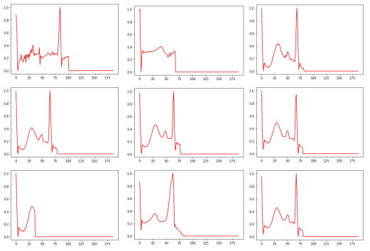
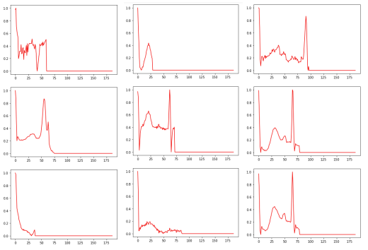
The data set is obtained by recording an electrocardiogram (ECG). For a patient with a normal heart rhythm, the ECG shows five waves:
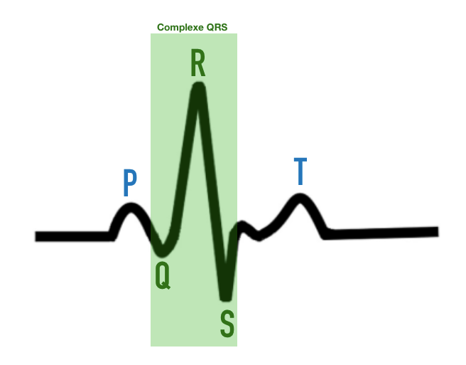
P wave: The P wave represents atrial depolarization, i.e. activation of the heart’s atria. When the sino-atrial (SA) node generates an electrical signal, the atria contract to propel blood to the ventricles. The P wave corresponds to this electrical activation of the atria, indicating their contraction.
QRS complex: The QRS complex is made up of three distinct waves: the Q wave, the R wave and the S wave. These waves represent ventricular depolarization, i.e. activation of the heart’s ventricles.
Q wave: The Q wave is a small negative wave that may be present in certain ECG leads. It indicates the onset of ventricular depolarization, generally in the interventricular septum (the wall separating the left and right ventricles).
R wave: The R wave is a positive wave that generally follows the Q wave. It represents continuous ventricular depolarization, indicating activation of the ventricles as a whole.
S wave: The S wave is a negative wave that follows the R wave. It also represents ventricular depolarization, and can vary in size and shape depending on the ECG and lead considered.
T wave: The T wave represents ventricular repolarization, i.e. the phase of electrical recovery of the ventricles after contraction. It indicates that the ventricles are ready to contract again during the next cardiac cycle. The T wave is generally a positive wave, but can also be negative under certain conditions.
These different waves (P, QRS and T) are essential for ECG interpretation and help assess the heart’s electrical activity, identifying possible cardiac abnormalities or dysfunctions. (1)
Conventionally, the term “normal sinus rhythm” (NSR) or “regular sinus rhythm” (RSR) indicates that not only do the P waves (which reflect sinus node activity) have a normal morphology, but that all other ECG measurements are also normal. The criteria therefore include the following:
- A regular rhythm.
- Heart rate between 60 and 100 beats per minute.
- Straight P waves, present in a 1:1 ratio, preceding each QRS complex.
- A PR interval of no more than 0.12 to 0.20 seconds.
- A QRS complex not exceeding 0.08 seconds.
Arrhythmia occurs when abnormalities occur in the P waves and QRS complex, particularly when the synchronization between atrial and ventricular contraction is altered. Normally, the P wave is always positive, so if this is not the case, it may indicate the presence of an abnormality.
For this use case, two data sets available on Kaggle will be used:
- mitbih_train: training set representing 877554 heart rhythms
- mitbih_test: test set representing 21892 heart rates
The two datasets contain 188 columns, the last of which indicates membership of the following five classes:
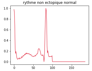
Class 0: Normal non-ectopic rhythm
This class represents normal, undisturbed cardiac rhythms. The data associated with this class are those in which the heart beats regularly and without abnormality.
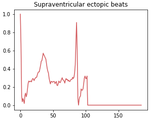
Class 1: Supraventricular ectopic beat
Supraventricular ectopic rhythms occur when abnormal electrical impulses form in the upper parts of the heart, such as the atria. This class includes abnormal heart rhythms that originate from P waves or a short PR interval or a narrow QRS complex or absence of complex.
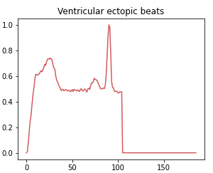
Class 2: Ventricular ectopic beat
Ventricular ectopic rhythms occur when abnormal electrical impulses form in the ventricles, the lower parts of the heart. This class includes abnormal heart rhythms that originate from R or S waves.
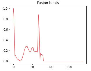
Class 3: Fusion beat
A fusion rhythm occurs when there is a combination of normal and abnormal electrical impulses occurring simultaneously in the heart. This class represents situations where the heart rhythm is a combination of normal and abnormal beats.
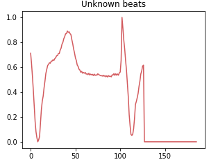
Class 4: Unknown beat
The class of unknown rhythms groups together data that cannot be classified with certainty in one of the other categories. This may be due to measurement errors, artifacts or infrequent or unidentified heartbeat patterns.
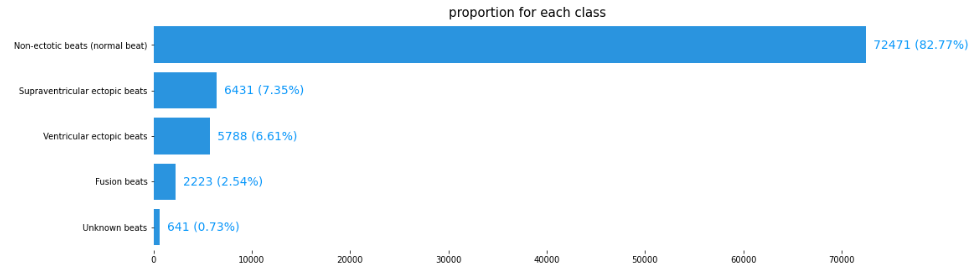
Breakdown of each class for the training set
Data pre-processing
Before any analysis, it is necessary to pre-process the dataset to enable the model to learn better.
Class rebalancing
In datasets of this type, whether used to predict faults for predictive maintenance or to detect credit card fraud, abnormal cases are rarely observed. This leads to class imbalance in the dataset. It is therefore necessary to find a method adapted to the use case to rebalance these classes. In this study, samples of under-represented classes are resampled to achieve the same sample size as the over-represented class.
For time series, class rebalancing requires a slightly different approach to conventional tabular data. When working with time series, it is essential to take into account the time dependency of the data to avoid introducing bias into the model during rebalancing.
There are a number of approaches to class rebalancing in time series:
SMOTE-TS generates new synthetic series by linearly interpolating between similar time series. This maintains the time dependency in the newly generated series.
Random sampling with replacement consists in increasing the number of samples from the minority class by randomly drawing samples from this class with replacement, i.e. by allowing duplication of existing samples.
In this use-case, the random draw is preferred. In fact, random sampling is a commonly used technique for oversampling time series.
It’s important to note, however, that the replacement draw can lead to a significant increase in the size of the minority class, which in turn can lead to overfitting.
Model selection and training
We used as a basis the paper [5], which presents an architecture composed of a succession of 1D convolution layers. And we adopted time series-to-image transformation techniques, which led us to use a model containing 2D convolutions.
For the purposes of our comparative study, we have retained the same architecture for the different models. Only the 1D convolution layers have been replaced by 2D convolutions, and the MaxPooling1D operations have been replaced by MaxPooling2D. This approach enables us to compare the performance of the different models while retaining a common basis for evaluation.
Training the CNN 1D Model
The model contains four blocks, with each block comprising the following layers:
- a 1D convolution layer based on a filter of size 32 (used to extract the important features of the input data in a window of size 32 pixels)
- MaxPool1D, where the maximum value of the window is selected to reduce the size of the output of the convolution layer
- and a Flatten layer that reduces multi-dimensional values to a single dimension.
Next, the model contains three dense layers and the last layer is the Softmax activation function which is used to return a membership score for each class.
This model uses a 1D convolution approach to extract important features from heart rate signals. MaxPool1D and Flatten layers are then used to reduce the dimensionality of the data and prepare it for the dense layers that will perform the final heart rate classification. This architecture is commonly used in signal processing tasks, as it efficiently captures important patterns in temporal data.
Training the CNN 2D Model
The second model uses a similar architecture to the previous model, but with one key difference: it is designed to process input data in the form of images. For this reason, the 1D convolution layers of the previous model are replaced by 2D convolution layers in this model, and the MaxPool1D layers are replaced by MaxPool2D layers.
The change in the dimensionality of the convolution and pooling layers is a necessary adaptation to process input data presented as images, which are two-dimensional structures (pixel arrays) rather than one-dimensional sequences like the heart rate data in the previous model.
The model contains four blocks, with each block comprising the following layers
- a 2D convolution layer where they have a filter of 32,
- a MaxPool2D layer where the maximum value of the window is selected
- and a Flatten layer that reduces the values to one dimension
Next, the model contains three dense layers and the last layer is the Softmax activation function which is used to return a membership score for each class.
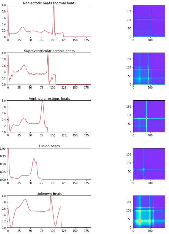
In order to use convolution-type models in 2D, the time series must be transformed into 2D. This can be done using a method called Gramian Angular Field.
Gramian Angular Field (GAF) is a transformation that allows a time series to be represented in the form of an image. It captures the angular relationships between the points in the time series. The resulting GAF image can then be used as input for models based on 2D convolutional neural networks. The advantages of this method are:
- Capture angular relationships between data points in the time series.
- Suitable for convolutional neural network (CNN) models.
- Can capture periodic and phase patterns in the time series.
- Some information in the time series may be lost in the transformation.
- Computations can be costly in terms of computing time and memory.
- Uniqueness of representation, there is no compression with loss of signal.
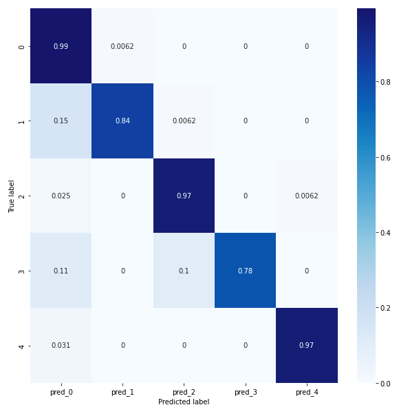
Results Comparison Between Conv 1D and Conv 2D models
In order to compare conv 1D and conv 2D we will study their confusion matrices. The confusion matrix for the conv1D model reveals that classes 0, 2 and 4 have a prediction score of at least 97%, indicating good accuracy. Classes 1 and 3 have a prediction score of at least 78% for the conv1D model, but less than 80%, which is still acceptable. However, it is important to ask why class 1 is predicted like class 0 at 15%. Similarly, class 3 is predicted as class 0 at 11%. Saimple helps to understand these prediction errors and why the network confuses a normal heart rhythm with supraventricular ectopic rhythms and fusion rhythms. It provides a better understanding of why these confusions occur and helps to identify the specific patterns that influence these erroneous predictions.
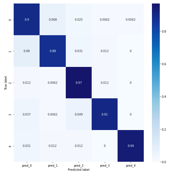
The confusion matrix for the conv 2D model reveals that overall the model achieves an accuracy of at least 88%, which is better than the conv1D model.
In cardiac arrhythmia detection, the choice between a 2D convolution model (Conv2D) and a 1D convolution model (Conv1D) depends on the specific characteristics of the data and how it is to be represented. Although 1D convolutional models are specifically designed to handle sequential data, 2D convolutional models can also exploit spatial and temporal relationships. They can capture patterns that repeat in both the temporal and spatial axes, which can be useful for time series with periodic or recurrent patterns. In the case of cardiac arrhythmias, this can be beneficial for detecting complex patterns in the ECG that indicate specific cardiac abnormalities.
However, it is important to note that using a Conv2D model can also have drawbacks. One potential disadvantage is that Conv2D models may require more data and have higher computational requirements than Conv1D models, due to the number of additional parameters needed to process the 2D data.
However, a Conv1D model may be sufficient to detect cardiac arrhythmia and can therefore limit the resources required to exploit the results. As the inputs are composed of a single ECG signal, Conv1D models can certainly capture the temporal variations of 1D signals sufficiently effectively.
Results obtained with Saimple
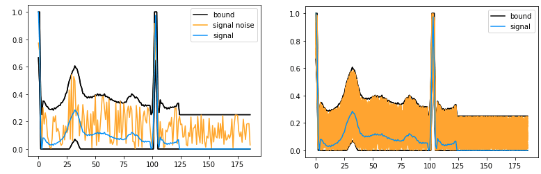
In order to evaluate the performance of the two models, a study can be carried out to measure the predictive stability of the models. To do this, abstract interpretation is used to model a set of possible variations in a time series in a single object, called an abstract envelope. This offers the advantage of grouping all the time series together and evaluating the behavior of the model on the whole in a single analysis. This envelope represents all the potential perturbations to a heart rate contained between two extreme time series. By bringing together this essential information in a single envelope, it is possible to gain an overall understanding of the variations in the model’s behavior over even very irregular versions of the heart rate, making it easier to analyze and detect any anomalies. This simplified approach increases efficiency while providing a complete overview for informed decision-making in cardiac health.
Example Of Input Perturbation
Time Series
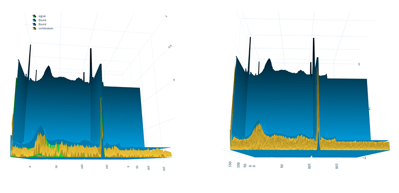
The time series transformed into an image using the GAF method with the help of 3D visualization
The performance of the two models, conv1D and conv2D, was evaluated using the full test dataset of 810 heartbeats to determine their ability to predict accurately. For this comparison, three abstract envelope volumes (corresponding to the maximum volume of noise considered) were selected: 1e-6, 1e-5 and 1e-4.
Initially, according to the results of the confusion matrix, the conv2D model seemed slightly superior in terms of performance. However, a crucial question remained: when faced with different levels of noise applied to the model, would the two models maintain their level of accuracy? This essential question raises the interest of verifying how each model behaves with different envelope thicknesses and assessing their robustness in the face of signal perturbations. An in-depth analysis of these aspects provides useful information for choosing the model best suited to the specific requirements of the application in question.
Using Saimple, it is possible to analyze the dominance values of a model’s prediction evaluation. Three terms are used: “Dominant”, “Dominated” and “Conflict”.
1. “Dominant” refers to an evaluation where the predicted class for all the time series considered by the model corresponds exactly to the true class. This means that the model has correctly identified the category to which the set of inputs considered belongs.
2. “Dominated” describes an evaluation where the class predicted by the model does not correspond to the true class. In other words, the model has made an error by predicting the wrong category for the set of inputs under consideration.
3. “Conflict” refers to an evaluation where the scores of the classes predicted by the model have equivalent values. In this situation, the model may be uncertain as to the appropriate class for the set of inputs, as several classes have similar scores.
These terms help to evaluate the performance of a model and to understand how it handles predictions for different classes of inputs. Analysis of these results can be useful in improving the model by identifying areas where it performs best and aspects where it may need adjustment to improve.
Result On A Volume Of 1 E-6
The graph below gives an overview of the frequency of occurrence of the terms “Dominant”, “Dominated” and “Conflict” for the true class, for the two models conv1D and conv2D.
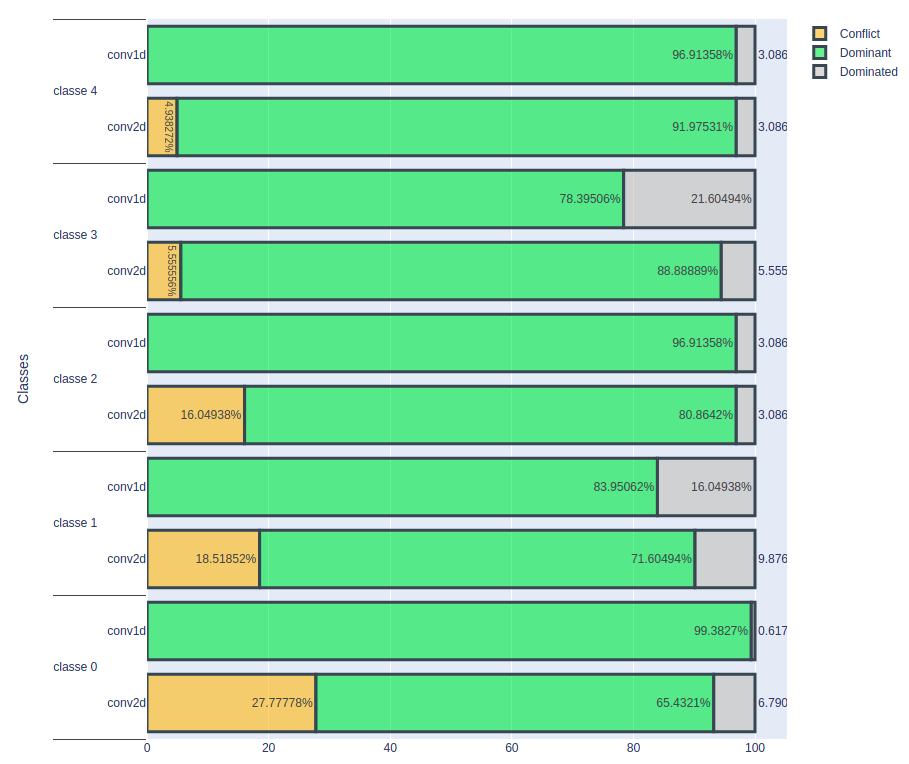
An important observation is that, for the conv1D model, the number of correctly classified cardiac rhythms remains constant. On the other hand, for the conv2D model, this number decreases, which suggests that this model has difficulty classifying some cardiac rhythms. The number of conflicting cases is also increasing. It seems that the input data is more sensitive to noise in the case of the conv2D model, resulting in lower classification accuracy for certain cardiac rhythms. These initial results indicate that the conv1D model is more stable than the conv2D model, at least under the current evaluation conditions. However, to reach more definitive conclusions, it would be advisable to deepen the analysis by examining more parameters and evaluation scenarios.
Result On A Volume Of 1 E-5
In the second experiment, a noise volume of 1e-5 was used.
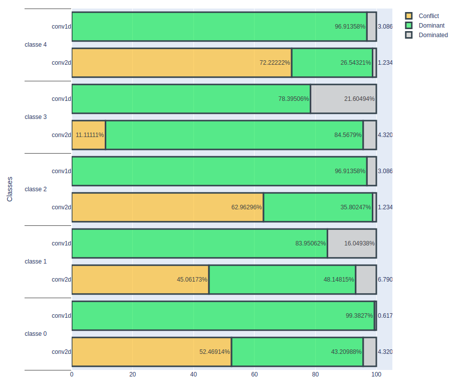
As expected, the conv2D model shows a sharp decrease in the number of correctly classified heartbeats. In contrast, the conv1D model maintains a constant number of correctly classified cardiac rhythms despite this level of noise. These results confirm that the conv1D model appears to be more stable and resilient to noise added to the data than the conv2D model.
However, the key question remains: up to what level of noise does the conv1D model remain stable? To answer this question, it would be relevant to continue experimenting by gradually increasing the noise volume and monitoring how the conv1D model reacts. This will make it possible to determine the threshold at which the accuracy of the conv1D model starts to decrease, thus providing crucial information for assessing the performance limits of this model in noisy data conditions. In summary, despite the good characteristics of the conv1D model, it is essential to explore its performance in greater depth in relation to the volume of noise in order to obtain a more accurate assessment of its robustness.
Result On A Volume Of 1 E-4
In this third experiment, a noise level of 1e-4 was applied to the data.
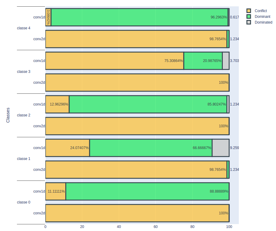
The results show that the conv2D model is no longer capable of correctly classifying cardiac rhythms at this noise level, showing a significant degradation in its performance.
In contrast, the conv1D model produced some interesting results. For class 0 cardiac rhythms (normal rhythm), the proportion of correctly classified cases seems to remain constant despite the noise. However, an intriguing observation is made for cardiac rhythms that are incorrectly classified at the outset: the model no longer seems to be able to classify them correctly. As for class 1 cardiac rhythms, the proportion correctly classified fell sharply, from 78% to 20%. This significant drop in performance raises questions about the reasons for this phenomenon.
For the other three classes, there was a slight decrease in the number of correctly classified heartbeats, indicating that the conv1D model is also beginning to show signs of sensitivity to noise at this level.
These results underline the importance of understanding how the conv1D model reacts to higher noise levels and highlight the need to determine the threshold at which its performance begins to degrade significantly. Further analysis of these results could provide information to assess the robustness of the conv1D model under noisy data conditions and identify the limits of its performance.
Review Of Previous Experiences
| Noise intensity | CONV1D Model | CONV2D Model |
|---|---|---|
| 1 E-6 | Maintains stability and a constant number of well-classified heartbeats ✅ | Shows a slight decrease in the number of well-classified cardiac rhythms ❌ |
| 1 E-5 | Maintains stability and a constant number of well-classified cardiac rhythms ✅ | Shows a sharp decrease in the number of well-classified heart rhythms ❌ |
| 1 E-4 | Shows a clear variation in the proportions of well-classified cardiac rhythms, particularly for cardiac rhythms that were initially poorly classified. ❌ | Unable to correctly classify heart rhythms at this noise level ❌ |
It is possible to consider adding noise in a targeted way to certain parts of the heartbeat to assess the robustness of a system in the face of specific variations linked to particular business contexts. This approach would make it possible to simulate realistic conditions and test a system’s ability to maintain its performance despite disturbances specific to a given application domain.
Analysis Of False Positives
In this study, we will focus our analysis on the cases where a normal heart rhythm is incorrectly classified as an abnormal rhythm and the results of the conv1D model. To do this, we will use the Saimple tool to identify rhythms that have encountered classification difficulties, characterised by the terms “dominated” and “conflict”, as a function of a specific noise level. The aim is to understand the underlying reasons for these prediction errors and to determine whether the model is vulnerable to different noise volumes. By analysing these cases of misclassification, we will be able to identify the distinctive patterns that influenced the mispredictions and assess the model’s ability to distinguish normal from abnormal heart rhythms in noisy conditions. This in-depth analysis will provide essential information for improving the accuracy and reliability of the cardiac arrhythmia detection model. We will also be able to find annotation errors using this approach.
Delta 1E-6 And Delta 1E-5
For these volumes of noise, only one rhythm is poorly classified (dominated) and none is in conflict.
On visual analysis of this heart rhythm classified as normal, it becomes clear that its recognition as a normal heart rhythm is erroneous. In fact, the presence of the QRS complex, which is essential for identifying a normal heart rhythm, is difficult to identify in this sequence. This observation raises doubts about the quality of the annotation of the data in the dataset. It is possible that some of the data has been incorrectly annotated, leading to errors in the predictions of the artificial intelligence model. A more thorough evaluation of the annotations and a more rigorous analysis of the data could resolve this problem and improve the accuracy of the detection of abnormal heart rhythms. Careful verification of the entire dataset is crucial to ensure the quality and reliability of the annotations, thereby guaranteeing more reliable and accurate results in the detection of cardiac arrhythmias.
Delta 1E-4
For this specific noise level, 18 heart rhythms were found to be classified as “conflicting”, meaning that the artificial intelligence model had difficulty determining with certainty the appropriate class for these rhythms. This situation occurs when the prediction scores for the different classes are similar, making the model uncertain as to which class each heartbeat belongs to. These results raise questions about the model’s ability to handle data in high noise conditions and highlight the need to improve its robustness to better handle these complex situations. Further analysis of these conflicting cardiac rhythms could provide important information for identifying the specific challenges posed by noise in the detection of cardiac arrhythmias and allow the model to be refined for more reliable and accurate performance.
The observations made on the misclassified cardiac rhythms challenge the quality of the annotation of the dataset. In fact, some heart rhythms are poorly annotated because they do not correspond to normal heart rhythms. More specifically, these rhythms show anomalies such as a lack of the QRS complex or a lack of visibility of the P or T waves. This clearly indicates a problem in the annotation of the dataset, which can greatly affect the relevance of the results obtained. The quality of the annotations in the data is an essential aspect of model training. Incorrectly annotated data can have a significant impact on the model’s performance, as it will learn from these inaccurate annotations and can lead to erroneous predictions.
Increasing the noise level has enabled us to highlight a large number of incorrectly annotated cardiac rhythms, which explains the loss of well-ranked cardiac rhythms for all the classes. It will then be possible to remove or correct the misannotated data identified in the set to improve the model’s performance. Saimple proved useful for detecting annotation problems in the dataset. By identifying conflicting and dominated rhythms, Saimple enabled us to identify weaknesses in the stability of the two models, particularly for the conv2D model, which showed a loss of performance at a noise level of 1e-6, which is relatively low.
In conclusion, although both models performed well overall for all the classes in the confusion matrix, they were unable to detect annotation errors in the dataset. Saimple proved to be a valuable tool for identifying these errors, based on the sensitivity of the models to varying volumes of noise. This makes it possible to address in a new semi-automated way the importance of having correctly annotated datasets in order to obtain good model performance. In addition, analysis with Saimple has highlighted areas of model weakness, which will help to guide future improvements and adjustments. For example, it will be possible to remove incorrectly annotated data to improve the robustness of cardiac arrhythmia detection models.
Conclusion
The use of artificial intelligence, in particular machine learning techniques such as 1D and 2D convolution models, offers a promising opportunity to improve the early detection of cardiac arrhythmias.
Arrhythmia is a common heart rhythm disorder that can lead to serious complications if not detected and treated early. AI can play a crucial role in this detection by analysing electrocardiographic signals and automatically identifying abnormalities in heart rhythm.
AI and arrhythmia detection algorithms are therefore increasingly present in the health applications of connected watches, enabling regular monitoring of the state of health of a large number of people.
Given the stakes involved, it is therefore necessary to ensure that arrhythmia detection algorithms are robust and explainable.
This study highlighted the importance of having a correctly annotated dataset in the field of cardiac arrhythmia detection. Observations made on misclassified cardiac rhythms reveal obvious annotation errors once the time series are isolated for analysis, with some cardiac rhythms incorrectly labelled as normal when they present anomalies such as a lack of QRS complex or absence of P or T waves. These annotation errors have a significant impact on the relevance of the results obtained, compromising the reliability of cardiac arrhythmia detection.
Experimentation with Saimple to increase the volume of noise detected a large number of incorrectly annotated cardiac rhythms. By identifying conflicting and dominated rhythms, Saimple highlighted the weaknesses of the two models, particularly for the conv2D model, which showed an early deterioration in its performance at a noise level of 1e-6, a relatively low level.
Thus, the use of Saimple made it possible to detect a weakness in the models and to offer ways of improving and adjusting them to increase the robustness of the cardiac arrhythmia detection models. By continuing to explore and fully exploit Saimple’s capabilities, it will be possible to further refine the models and provide more effective tools for the early and accurate detection of cardiac arrhythmias, thereby helping to improve the management and treatment of patients with cardiac disorders.
In short, this study illustrates how artificial intelligence can be a valuable tool in the detection of cardiac arrhythmias, but also the importance of understanding the performance and limitations of these models for effective and safe clinical application.
References
Authors


